Dimensionality Reduction

The performance of machine learning algorithms can degrade with too many input variables. Having a large number of dimensions in the feature space can mean that the volume of that space is very large, and in turn, the points that we have in that space (rows of data) often represent a small and non-representative sample. This can dramatically impact the performance of machine learning algorithms fit on data with many input features, generally referred to as the curse of dimensionality. This reduces the number of dimensions of the feature space, hence the name dimensionality reduction.

Dimensionality Reduction

Dimensionality reduction refers to techniques for reducing the number of input variables in training data. Fewer input dimensions often mean correspondingly fewer parameters or a simpler structure in the machine learning model, referred to as degrees of freedom. A model with too many degrees of freedom is likely to overfit the training dataset and therefore may not perform well on new data. There are a large number of techniques to reduce the dimensions such as forward/backward feature selection or combining the dimensions together by calculating weighted average of the correlated features.

Linear Discriminant Analysis

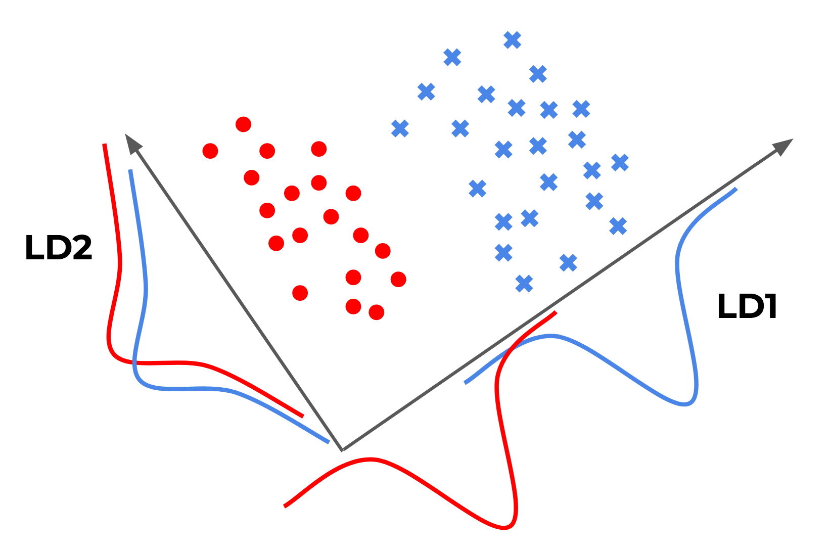
Linear Discriminant Analysis, or LDA, is a linear machine learning algorithm used for multi-class classification. LDA is used for compressing supervised data. When we have a large set of features (classes), and our data is normally distributed and the features are not correlated with each other then we can use LDA to reduce the number of dimensions. LDA is a generalised version of Fisher’s linear discriminant.

Linear Discriminant Analysis seeks to best separate (or discriminate) the samples in the training dataset by their class value. Specifically, the model seeks to find a linear combination of input variables that achieves the maximum separation for samples between classes (class centroids or means) and the minimum separation of samples within each class.

from sklearn.lda import LDA
my_lda = LDA(n_components=3)
lda_components = my_lda.fit_transform(X_train, Y_train)

Principal Component Analysis

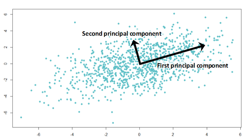
PCA can be defined as the orthogonal projection of the data onto a lower dimensional linear space, known as the principal subspace, such that the variance of the projected data is maximized. They are mainly used for compressing unsupervised data. PCA is a very useful technique that can help de-noise and detect patterns in data. PCA is used in reducing dimensions in images, textual contents and in speech recognition systems.

from sklearn.decomposition import PCA
pca_classifier = PCA(n_components=3)
my_pca_components = pca_classifier.fit_transform(X_train)

Kernel Principal Component Analysis

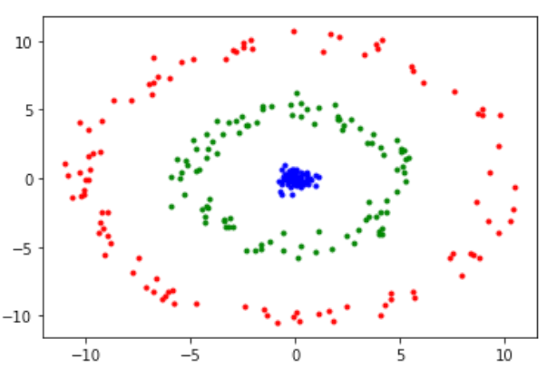
When we have non-linear features then we can project them onto a larger feature set to remove their correlations and to make them linear. Essentially, non-linear data is mapped and transformed onto a higher-dimensional space. Then PCA is used to reduce the dimensions. However, one downside of this approach is that it is computationally very expensive.

Just like in PCA, we first compute variance-covariance matrix and then eigen vectors and eigen values are prepared with the highest variance to compute principal components. We then compute kernel matrix. This requires us to construct a similarity matrix. The matrix is then decomposed via creating eigen values and eigen vectors.

from sklearn.decomposition import KernelPCA
kpca = KernelPCA(n_components=2,kernel='rbf', gamma=45)
kpca_components = kpca.fit_transform(X)