Support Vector Machine

The support vector machine is a generalization of a classifier called maximal margin classifier. The maximal margin classifier is simple, but it cannot be applied to the majority of datasets, since the classes must be separated by a linear boundary. That is why the support vector classifier was introduced as an extension of the maximal margin classifier, which can be applied in a broader range of cases. Finally, support vector machine is simply a further extension of the support vector classifier to accommodate non-linear class boundaries.

Maximal Margin Classifier

This method relies on separating classes using a hyperplane. A hyperplane is a line that splits the input variable space. In SVM, a hyperplane is selected to best separate the points in the input variable space by their class, either class 0 or class 1. In two-dimensions you can visualize this as a line and let’s assume that all of our input points can be completely separated by this line. For example: \(B_0 + (B_1 * X_1) + (B_2 * X_2) = 0\)

Where the coefficients (B1 and B2) that determine the slope of the line and the intercept (B0) are found by the learning algorithm, and X1 and X2 are the two input variables.

You can make classifications using this line. By plugging in input values into the line equation, you can calculate whether a new point is above or below the line.

• Above the line, the equation returns a value greater than 0 and the point belongs to the first class (class 0).
• Below the line, the equation returns a value less than 0 and the point belongs to the second class (class 1).
• A value close to the line returns a value close to zero and the point may be difficult to classify.
• If the magnitude of the value is large, the model may have more confidence in the prediction.

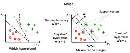
In general, if the data can be perfectly separated using a hyperplane, then there is an infinite number of hyperplanes, since they can be shifted up or down, or slightly rotated without coming into contact with an observation.

That is why we use the maximal margin hyperplane or optimal separating hyperplane which is the separating hyperplane that is farthest from the observations. We calculate the perpendicular distance from each training observation given a hyperplane. This is known as the margin. Hence, the optimal separating hyperplane is the one with the largest margin.

Soft Margin Classifier

The constraint of maximizing the margin of the line that separates the classes must be changed over the time. This is often called the soft margin classifier. This change allows some points in the training data to violate the separating line.

A tuning parameter is introduced called simply C that defines the magnitude of the wiggle allowed across all dimensions. The C parameters defines the amount of violation of the margin allowed. A C=0 is no violation and we are back to the inflexible Maximal-Margin Classifier described above. The larger the value of C the more violations of the hyperplane are permitted.

During the learning of the hyperplane from data, all training instances that lie within the distance of the margin will affect the placement of the hyperplane and are referred to as support vectors. And as C affects the number of instances that are allowed to fall within the margin, C influences the number of support vectors used by the model.

• The smaller the value of C, the more sensitive the algorithm is to the training data (higher variance and lower bias).
• The larger the value of C, the less sensitive the algorithm is to the training data (lower variance and higher bias).

SVM Kernels

The SVM algorithm is implemented in practice using a kernel. The learning of the hyperplane in linear SVM is done by transforming the problem using some linear algebra. The equation for making a prediction for a new input using the dot product between the input (x) and each support vector (xi) is calculated as follows: \(f(x) = B_0 + \sum{(a_i * (x,x_i))}\)

Linear Kernel

The kernel defines the similarity or a distance measure between new data and the support vectors. The dot product is the similarity measure used for linear SVM or a linear kernel because the distance is a linear combination of the inputs. The dot-product is called the kernel and can be re-written as: \(K(x, x_i) = \sum{(x * x_i)}\)

Polynomial Kernel

Instead of the dot-product, we can use a polynomial kernel, for example: \(K(x,x_i) = 1 + \sum{(x * x_i)^d}\)

Where the degree of the polynomial must be specified by hand to the learning algorithm. When d=1 this is the same as the linear kernel. The polynomial kernel allows for curved lines in the input space.

Radial Kernel

Finally, we can also have a more complex radial kernel. For example: \(K(x,x_i) = \exp (-\gamma * \sum{((x – x_i)^2)}\)

Where gamma is a parameter that must be specified to the learning algorithm. A good default value for gamma is 0.1, where gamma is often 0 < gamma < 1. The radial kernel is very local and can create comp

Data Preparation for SVM

This section lists some suggestions for how to best prepare your training data when learning an SVM model.

• Numerical Inputs: SVM assumes that your inputs are numeric. If you have categorical inputs you may need to covert them to binary dummy variables (one variable for each category).
• Binary Classification: Basic SVM as described in this post is intended for binary (two-class) classification problems. Although, extensions have been developed for regression and multi-class classification.