K Nearest Neighbour

K Nearest Neighbour (KNN) works by choosing the best $k$ of neighbour. Neighbour by definition is a person living near or next door to the speaker or person referred to. In this context, the neighbour is the data. Predictions in KNN are made with a new instance $x$ by searching through the entire training set for the $k$ most similar instances (the neighbors) and summarizing the output variable for those $k$ instances. For regression this might be the mean output variable, in classification this might be the mode (or most common) class value.

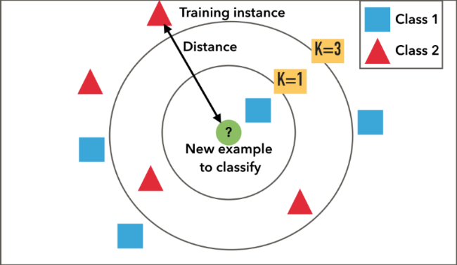
When we trained the KNN on training data, it took the following steps for each data sample:

1. Calculate the distance between the data sample and every other sample with the help of a method such as Euclidean.
2. Sort these values of distances in ascending order.
3. Choose the top $k$ (nearest distance according to your own distance method) values from the sorted distances.
4. Assign the class to the sample based on the most frequent class in the above K values.

The computational complexity of KNN increases with the size of the training dataset. For very large training sets, KNN can be made stochastic by taking a sample from the training dataset from which to calculate the K-most similar instances.

KNN has been around for a long time and has been very well studied. As such, different disciplines have different names for it, for example:

• Instance-Based Learning: The raw training instances are used to make predictions. As such KNN is often referred to as instance-based learning or a case-based learning (where each training instance is a case from the problem domain).
• Lazy Learning: No learning of the model is required and all of the work happens at the time a prediction is requested. As such, KNN is often referred to as a lazy learning algorithm.
• Non-Parametric: KNN makes no assumptions about the functional form of the problem being solved. As such KNN is referred to as a non-parametric machine learning algorithm.

KNN Distance Metrics

To determine which of the $k$ instances in the training dataset are most similar to a new input a distance measure is used. For real-valued input variables, the most popular distance measure is Euclidean distance. \(EuclideanDistance(x, x_i) = \sqrt{ \sum{ (x_j – x_{ij})^2} }\) Other popular distance measures include:

• Hamming Distance: Calculate the distance between binary vectors.
• Manhattan Distance: Calculate the distance between real vectors using the sum of their absolute difference. Also called City Block Distance.
• Minkowski Distance: Generalization of Euclidean and Manhattan distance

There are many other distance measures that can be used, such as Tanimoto, Jaccard, Mahalanobis and cosine distance. You can choose the best distance metric based on the properties of your data. If you are unsure, you can experiment with different distance metrics and different values of $k$ together and see which mix results in the most accurate models. Particularly, in Scikit-Learn you can use

Metrics intended for real-valued vector spaces:

identifier	class name	args	distance function
“euclidean”	EuclideanDistance		sqrt(sum((x - y)^2))
“manhattan”	ManhattanDistance		sum(|x - y|)
“chebyshev”	ChebyshevDistance		max(|x - y|)
“minkowski”	MinkowskiDistance	p	sum(|x - y|^p)^(1/p)
“wminkowski”	WMinkowskiDistance	p, w	sum(|w * (x - y)|^p)^(1/p)
“seuclidean”	SEuclideanDistance	V	sqrt(sum((x - y)^2 / V))
“mahalanobis”	MahalanobisDistance	V or VI	sqrt((x - y)' V^-1 (x - y))

Metrics intended for two-dimensional vector spaces: Note that the haversine distance metric requires data in the form of [latitude, longitude] and both inputs and outputs are in units of radians.

identifier	class name	distance function
“haversine”	HaversineDistance	2 arcsin(sqrt(sin^2(0.5*dx) + cos(x1)cos(x2)sin^2(0.5*dy)))

Metrics intended for integer-valued vector spaces: Though intended for integer-valued vectors, these are also valid metrics in the case of real-valued vectors.

identifier	class name	distance function
“hamming”	HammingDistance	N_unequal(x, y) / N_tot
“canberra”	CanberraDistance	sum(|x - y| / (|x| + |y|))
“braycurtis”	BrayCurtisDistance	sum(|x - y|) / (sum(|x|) + sum(|y|))

Metrics intended for boolean-valued vector spaces: Any nonzero entry is evaluated to “True”. In the listings below, the following abbreviations are used:

• N : number of dimensions
• NTT : number of dims in which both values are True
• NTF : number of dims in which the first value is True, second is False
• NFT : number of dims in which the first value is False, second is True
• NFF : number of dims in which both values are False
• NNEQ : number of non-equal dimensions, NNEQ = NTF + NFT
• NNZ : number of nonzero dimensions, NNZ = NTF + NFT + NTT

identifier	class name	distance function
“jaccard”	JaccardDistance	NNEQ / NNZ
“matching”	MatchingDistance	NNEQ / N
“dice”	DiceDistance	NNEQ / (NTT + NNZ)
“kulsinski”	KulsinskiDistance	(NNEQ + N - NTT) / (NNEQ + N)
“rogerstanimoto”	RogersTanimotoDistance	2 * NNEQ / (N + NNEQ)
“russellrao”	RussellRaoDistance	NNZ / N
“sokalmichener”	SokalMichenerDistance	2 * NNEQ / (N + NNEQ)
“sokalsneath”	SokalSneathDistance	NNEQ / (NNEQ + 0.5 * NTT)

Fake Neighbour Problem

When the value of $k$ or the number of neighbors is too low, the model picks only the values that are closest to the data sample, thus forming a very complex decision boundary. Such a model fails to generalize well on the test data set, thereby showing poor results.

The problem can be solved by tuning the value of n_neighbors parameter. As we increase the number of neighbors, the model starts to generalize well, but increasing the value too much would again drop the performance. Therefore, it’s important to find an optimal value of K, such that the model is able to classify well on the test data set. Let’s observe the train and test accuracies as we increase the number of neighbors.

Curse of Dimensionality

KNN works well with a small number of input variables (p), but struggles when the number of inputs is very large. Each input variable can be considered a dimension of a p-dimensional input space. For example, if you had two input variables x1 and x2, the input space would be 2-dimensional. As the number of dimensions increases the volume of the input space increases at an exponential rate. In high dimensions, points that may be similar may have very large distances. All points will be far away from each other and our intuition for distances in simple 2 and 3-dimensional spaces breaks down. This might feel unintuitive at first, but this general problem is called the “Curse of Dimensionality“.

Best Prepare Data for KNN

Rescale Data

KNN performs much better if all of the data has the same scale. Normalizing your data to the range [0, 1] is a good idea. It may also be a good idea to standardize your data if it has a Gaussian distribution.

Address Missing Data

Missing data will mean that the distance between samples can not be calculated. These samples could be excluded or the missing values could be imputed.

Lower Dimensionality

KNN is suited for lower dimensional data. You can try it on high dimensional data (hundreds or thousands of input variables) but be aware that it may not perform as well as other techniques. KNN can benefit from feature selection that reduces the dimensionality of the input feature space.