Decision Tree

Decision trees are very popular machine learning algorithm. They are popular because a variety of reasons, being their interpretability probably their most important advantage. They can be trained very fast and are easy to understand, which opens their possibilities to frontiers far beyond scientific walls. Nowadays, Decision Tree are very popular in business environments and their usage is also expanding to civil areas, where some applications are raising big concerns.

Classification and Regression Tree

Classification and Regression Trees (CART)introduced by Leo Breiman to refer to Decision Tree algorithms that can be used for classification or regression predictive modeling problems. The representation of the CART model is a binary tree. This is the same binary tree from algorithms and data structures, nothing too fancy (each node can have zero, one or more child nodes).

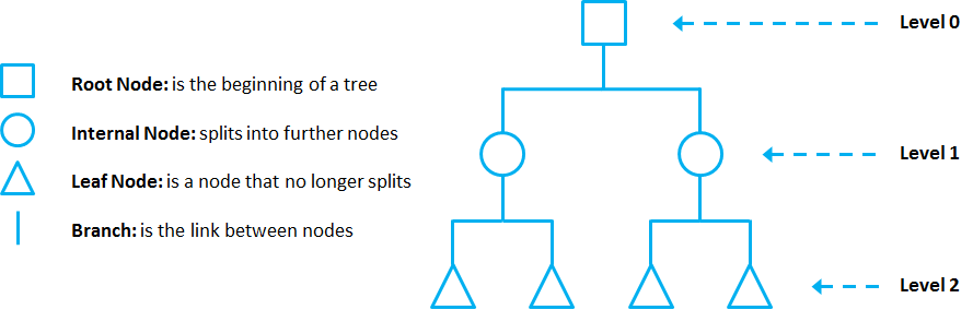
Decision Tree are composed of nodes, branches and leafs. Each node represents an attribute (or feature), each branch represents a rule (or decision), and each leaf represents an outcome. The depth of a Tree is defined by the number of levels, not including the root node.

Decision Tree apply a top-down approach to data, so that given a data set, they try to group and label observations that are similar between them, and look for the best rules that split the observations that are dissimilar between them until they reach certain degree of similarity.

The splitting can be binary (which splits each node into at most two sub-groups, and tries to find the optimal partitioning), or multiwayDeciare preferred over super complex ones, since they are easier to understand and they are less likely to fall into overfitting.

The split with the best cost (lowest cost because we minimize cost) is selected. All input variables and all possible split points are evaluated and chosen in a greedy manner based on the cost function.

• Regression: The cost function that is minimized to choose split points is the sum squared error across all training samples that fall within the rectangle.
• Classification: The cost function is used which provides an indication of how pure the nodes are, where node purity refers to how mixed the training data assigned to each node is.

Gini Impurity

In the case of Classification Trees, CART algorithm uses a metric called Gini Impurity to create decision points for classification tasks. Gini Impurity is a measurement of the likelihood of an incorrect classification of a new instance of a random variable, if that new instance were randomly classified according to the distribution of class labels from the data set. A Gini impurity gives an idea of how good a split is by how mixed the classes are in the two groups created by the split. A perfect separation results in a Gini score of 0, whereas the worst case split that results in 50/50 classes in each group result in a Gini score of 0.5 (for a 2 class problem).

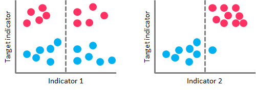
On the left-hand side, a high Gini Impurity value leads to a poor splitting performance. On the right-hand side, a low Gini Impurity value performs a nearly perfect splitting

Least Squared Deviation

In the case of Regression Trees, CART algorithm looks for splits that minimize the Least Square Deviation (LSD), choosing the partitions that minimize the result over all possible options. The LSD (sometimes referred as “variance reduction”) metric minimizes the sum of the squared distances (or deviations) between the observed values and the predicted values. The difference between the predicted and observed values is called “residual”, which means that LSD chooses the parameter estimates so that the sum of the squared residuals is minimized.

Pruning

As the number of splits in DTs increase, their complexity rises. In general, simpler DTs are preferred over super complex ones, since they are easier to understand and they are less likely to fall into overfitting. In other words, the model learns the detail and noise (irrelevant information or randomness in a dataset) in the training data to the extent that it negatively impacts the performance of the model on new data. This means that the noise or random fluctuations in the training data is picked up and learned as concepts by the model.

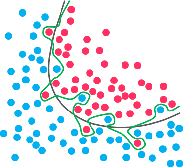
While the black line fits the data well, the green line is overfitting. Under this condition, your model works perfectly well with the data you provide upfront, but when you expose that same model to new data, it breaks down. It’s unable to repeat its highly detailed performance.

Pruning is a technique used to deal with overfitting, that reduces the size of DTs by removing sections of the Tree that provide little predictive or classification power. The goal of this procedure is to reduce complexity and gain better accuracy by reducing the effects of overfitting and removing sections of the DT that may be based on noisy or erroneous data. There are two different strategies to perform pruning on DTs:

• Pre-prune: When you stop growing DT branches when information becomes unreliable.
• Post-prune: When you take a fully grown DT and then remove leaf nodes only if it results in a better model performance. This way, you stop removing nodes when no further improvements can be made.

Ensemble Methods

Ensemble methods combine several DTs to improve the performance of single DTs, and are a great resource to get over the problems already described. The idea is to train multiple models using the same learning algorithm to achieve superior results. The 2 most common techniques to perform ensemble Decision Tree are Bagging and Boosting.

Bagging

Bagging (or Bootstrap Aggregation) is used when the goal is to reduce the variance of a DT. Variance relates to the fact that DTs can be quite unstable because small variations in the data might result in a completely different Tree being generated. So, the idea of Bagging is to solve this issue by creating in parallel random subsets of data (from the training data), where any observation has the same probability to appear in a new subset data.

Next, each collection of subset data is used to train DTs, resulting in an ensemble of different DTs. Finally, an average of all predictions of those different DTs is used, which produces a more robust performance than single DTs. Random Forest is an extension over Bagging, which takes one extra step: in addition to taking the random subset of data, it also takes a random selection of features rather than using all features to grow DTs.

Boosting

Boosting is another technique that creates a collection of predictors to reduce the variance of a DT, but with a different approach. It uses a sequential method where it fits consecutive DTS, and at every step, tries to reduce the errors from the prior Tree. With Boosting techniques, each classifier is trained on data, taking into account the previous classifier success. After each training step, the weights are redistributed based on the previous performance.

This way, misclassified data increases its weights to emphasize the most difficult cases, so that subsequent DTs will focus on them during their training stage and improve their accuracy. Unlike Bagging, in Boosting the observations are weighted and therefore some of them will take part in the new subsets of data more often. As a result of this process, the combination of the whole sets improves the performance of DTs.