Handling Imbalance Data

Data imbalance usually reflects an unequal distribution of classes within a dataset. In class imbalance, one trains on a dataset that contains a large number of instances of one type, for example, malicious files, and only a few instances of other types, for example, clean files. The most common example, in a credit card fraud detection dataset, most of the credit card transactions are not fraud and very few classes are fraud transactions. This leaves us with something like a 99:1 ratio between the fraud and non-fraud classes.

Now let’s talk about how to handle imbalance data.

Use different metrics

Imagine our training data is the one illustrated in the graph above. If accuracy is used to measure the goodness of a model, a model which classifies all testing samples into “0” will have an excellent accuracy (99.8%), but obviously, this model won’t provide any valuable information for us.

In this case, other alternative evaluation metrics can be applied such as:

• Precision/Specificity: how many selected instances are relevant.
• Recall/Sensitivity: how many relevant instances are selected.
• F1 score: harmonic mean of precision and recall.
• MCC: correlation coefficient between the observed and predicted binary classifications.
• AUC: the relation between true-positive rate and false-positive rate.

Resampling

These approaches change the data distribution by either undersampling the majority classes or oversampling the minority classes to balance the data distribution.

In undersampling, one can remove instances from the majority class, whereas in oversampling, duplicates of the minority class instances are added to the learning set. Generally, it is advisable to resort to undersampling when you have a large number of training samples and use oversampling when the number of training examples is small.

Both of these two techniques, however, have drawbacks. Undersampling can lead to the loss of useful and potentially discriminative information about the majority class, whereas oversampling cause overfitting. This overfitting while oversampling can be addressed using approaches such as Synthetic Minority Over-sampling Technique (SMOTE) and Adaptive Synthetic Sampling (ADASYN). We can talk about sampling techniques in the next post.

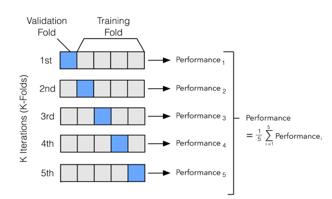
Cross-Validation Usage

It is noteworthy that cross-validation should be applied properly while using an over-sampling method to address imbalance problems.

Keep in mind that over-sampling takes observed rare samples and applies bootstrapping to generate new random data based on a distribution function. If cross-validation is applied after over-sampling, basically what we are doing is overfitting our model to a specific artificial bootstrapping result. That is why cross-validation should always be done before over-sampling the data, just as how feature selection should be implemented. Only by resampling the data repeatedly, randomness can be introduced into the dataset to make sure that there won’t be an overfitting problem.

Ensembling the Models

Ensemble methods use multiple learning algorithms and techniques to obtain better performance than what could be obtained from any of the constituent learning algorithms alone.

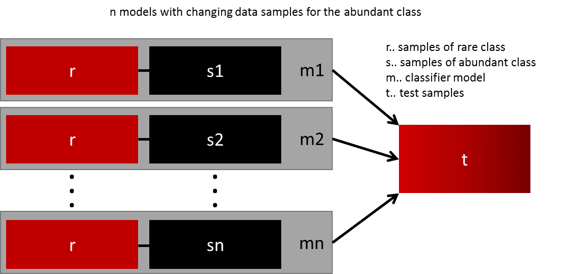
One easy best practice is building n models that use all the samples of the rare class and n-differing samples of the abundant class. Given that you want to ensemble 10 models, you would keep e.g. the 1.000 cases of the rare class and randomly sample 10.000 cases of the abundant class. Then you just split the 10.000 cases into 10 chunks and train 10 different models.

When using ensemble classifiers, bagging methods become popular and it works by building multiple estimators on a different randomly selected subset of data. In the scikit-learn library, there is an ensemble classifier named BaggingClassifier. However, this classifier does not allow to balance of each subset of data. Therefore, when training on imbalanced data set, this classifier will favour the majority classes and create a biased model.